In this article we considerљcalculationљof discrete Laplacian for 1D arrays usingљpython/numpy/scipy. We introduceљthe sparse matrix technique that is rather efficient for computation of certain types of diffusion PDE.
Discrete Laplacian in case of one dimensional space
First, let us consider the simplest case of diffusion in the linear reactor.
We suppose that the reactor contains only four cells, therefore we can write substance vector in form:
Let us denote the distance between adjacent cells asљh and use periodicљboundary conditions. Then the discrete Lapplacian is calculated as:
")
Thus, action of theљLaplacian operator on the vector in discrete space is equivalent to its multiplication by the matrix of discrete Laplacian:
 = \frac{1}{h^2} \left( \begin{matrix} v_2-2v_1+v_4 \\ v_3-2v_2+v_1 \\ v_4-2v_3+v_2 \\ v_1-2v_4-v_3 \end{matrix} \right)")
Matrix of discrete 1-dimensional Laplacian canљbe simplifiedљfor Neumann boundary conditions:
 \vec{v}")
… or for Dirichlet boundary conditions:
It is clear that such matrix can be easilyљbuilt for any number of cells.
")
")
Sparse matrix python syntax
Let us note that the matrix of discrete Laplacian is always sparse due to the large numberљof zero elements. Therefore we can useљtheљsparse matrix technique. It is implemented in scipy.sparse library, so we need to import it:
import scipy.sparse as sp
Sparse matrices canљbe stored in differentљformats. You can find the detailed description of this formats in the following presentation of series «Advanced Numerical Algorithms in scipy/numpy» [reference]. In short, there are two kinds of sparse containers: the one used for element assignment (COO, LIL) and the one used for linear algebra (CSR, CSC). You can easily convert one to another. For instance:
mm = sp.lil_matrix((10000,10000), dtype=float32)
mm[100,2345] = 12.5
Often sparse matrices have all the diagonal elements different from zero (that is exactly our case). Inљthis case we can use a special function spdiags. We number matrix diagonals as follows: the main diagonal has number «0», theљdiagonals under the main diagonal has number «-1», the diagonal above main diagonal has number «+1», etc. All diagonals are considered to beљgiven in 1xN form but «-1» diagonal is shifted to the left and «+1» is shifted to the right. For instance, the code
diag1 = [1]*10000
diag2 = [2]*10000
mm = sp.spdiags([ diag2, diag1, diag2], [ -1, 0, 1], 10000, 10000)
… forms a tridiagonal matrix with «1» at the main diagonal and «2» at adjacent diagonals. Next, we can set values of some cells explicitly:
mm = mm.tolil() # LIL form suites for exact cell settings
mm[9999,0]=1
mm[0,9999]=1
As we want to perform vector-matrix multiplication further we should convert our sparse matrix into CSR form:
mm = mm.tocsr()
m = np.random.randn(10000)
n = mm.dot(m) # matrix-vector multiplication
Implementation of discrete Laplacian using sparse matrices
Let us implement the code for building sparse matrix of theљdiscrete Laplacian with Neumann boundary conditions:
def gen_laplacian(num):
љљљ data1 = [-2]*num
љљљ data1[0] = -1
љљљ data1[-1] = -1
љљљ data2 = [1]*num
љљљ L = sp.spdiags([ data2, data1, data2 ], [-1, 0, 1], num, num)
    return L.tocsr()
The main diagonal consists of «-2» elements and we put «-1» elements at the ends. To apply periodicљboundary conditions we should include «1» to the bottom left and the upper right corners of the whole matrix. We can do it using theљLIL form:
def gen_laplacian_pbc(num):
љљљ data1 = [-2]*num
љљљ data2 = [1]*num
љљљ L = sp.spdiags([ data2, data1, data2 ], [-1, 0, 1], num, num).tolil()
    L[num-1,0] = 1
    L[0,num-1] = 1
    return L.tocsr()
Now one can apply Laplace filter:
u = numpy.randn(10000)
L = gen_laplacian_pbc(10000)
u_transformed = L.dot(u)
or inverse Laplace filter:
u_inv = lg.spsolve(L,u)
Note, that for usingљspsolve oneљshould importљlinear algebra package for sparse matrices:
imprt scipy.sparse.linalg as lg
Let us use the discrete Laplacian for computing the second order derivative and also to solve the reverse problem — calculation of double integral.
First, we define x array and renormalize the Laplacian according to the number of points and the interval size h (not to forget!):
x = linspace(0,8*pi,10000)
L = gen_laplacian_circ(10000)*(10000/8/pi)**2
We use periodicљboundary conditions and thus, our function should be a smooth intersection of 8?љ? 0 points. We use 8?-periodic function:
u = sin(x)*x*(8*pi-x)
Finally,љwe can plot both double integral and second order derivatives with just one line of code:
plot(x,L.dot(u))
plot(x,lg.spsolve(L,u))
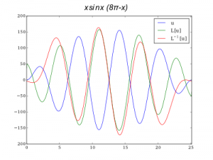
Interval was divided into 10000 points. Periodicљboundary conditions were used.
Simple benchmark:љ Sparse vs Dense
This simple code implements the explicit scheme for solving Fick equation. It performes one thousand matrix-vector multiplications of discrete laplacian matrix and vector u.
def sparse(sparsed, Nli):
   for N in Nli:
      L = gen_laplacian(N)
      if not sparsed:
          L = L.toarray() # makes L matrix dense
      start = time.clock() # matrix construction is not included into time estimation
      u0 = numpy.abs(numpy.random.randn(N))
      u = copy(u0)
      for i in range(1000):
          u += 0.01*L.dot(u)
      stop = time.clock()
      print 'For %d array we used %.4f sec.' % (N, (stop-start))

print 'Sparsed statistics'
sparse(True, [10, 100, 1000, 10000, 100000])
print 'Full matrix statistics'
sparse(False, [10, 100, 1000, 2000, 3000])
My machine (i7-2640M CPU @ 2.80GHz) returns the following (numpy version 1.10.1 and scipy version 0.14.0):
Sparsed statistics
For 10 array we used 0.0164 sec.
For 100 array we used 0.0170 sec.
For 1000 array we used 0.0253 sec.
For 10000 array we used 0.0972 sec.
For 100000 array we used 1.2338 sec.
Full matrix statistics
For 10 array we used 0.0038 sec.
For 100 array we used 0.0234 sec.
For 1000 array we used 2.3979 sec.
For 2000 array we used 9.7725 sec.
For 3000 array we used 24.7091 sec.
We can see that sparse matix-vector multiplication hasљapproximatelyљO(N) complexity whereas dense matrix-vector multiplication complexity is close to O(N2).